Bridge in Excel (waterfall)

Ever needed to compare two results, like EBIT or net sales, and explain the variations between them? That’s where a bridge comes in handy!

Here’s how to build one:

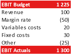
  • Create a table: Start with a table that lists the starting point on the first row, the end point on the last row, and the various variations in between. You may need an “Other” line to ensure the bridge is complete.
  • Insert the Bridge: Select the table, go to Insert > Waterfall (Alt > N > I1 > Enter)
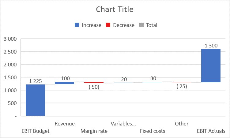
  • Customize the Appearance: Set the title in bold, delete the gridlines and borders (Alt > JA > SO > N > Enter). Change the colors in the legend to green for increase, red for decrease, and dark gray for total.
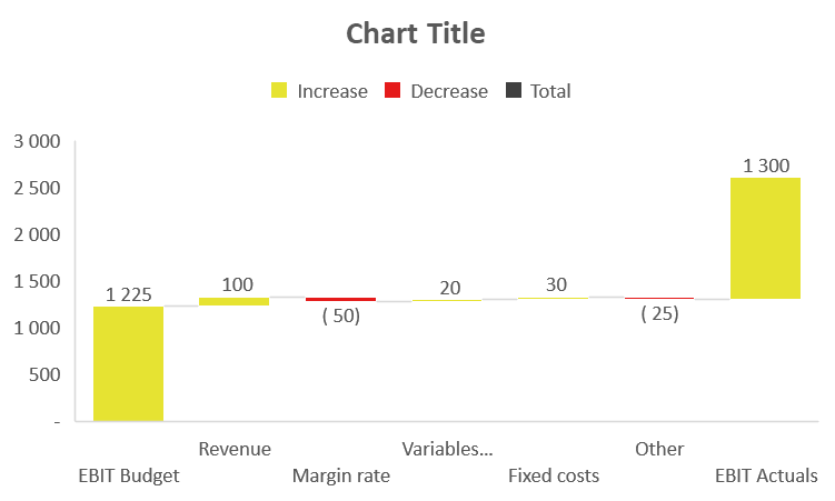
  • Final Touches: Delete the legend. Double-click the first and last columns, then right-click > Set as Total. You should obtain something similar to this:
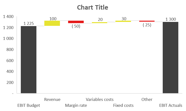
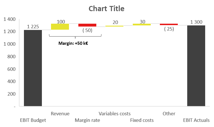
You can now copy the bridge image into PowerPoint, position it on the left, and add commentaries on the right. For specific comments, consider adding brackets such as in the example below:
Open a second Excel window

This tip can save you a lot of time and headaches.

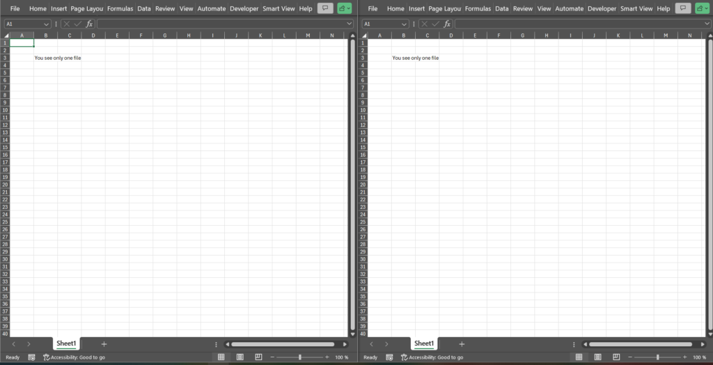
Let’s say you have an Excel file with 50 sheets, and you want to work on a formula in the first sheet using data from the last sheet. Navigating between sheets can be cumbersome. Creating a new instance of the same Excel file allows you to switch back and forth between sheets easily. Here’s how to do it:

  • Go to View > New Window (or press Alt > W > N).

Now, it’s like you have two instances of the same Excel file open. On one instance, go to the first sheet, and on the other, go to the last sheet.

And here’s where the magic happens: you can simply press Alt + Tab to switch between sheets.

You can even open more than two windows of the same Excel file. I use this all the time.

Insert a table in a PowerPoint

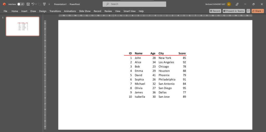
You’ve worked on a table and want to insert it nicely into your PowerPoint. Here’s how to do it:

  1. In Excel, select the table and copy it.
  2. In PowerPoint, Home > Paste > Image (or Alt > H > V > U).

Once pasted, never resize the image from the left/right or top/bottom sides, as this will distort the image ratio and make it look unappealing. Instead, always use one of the four corners or use Shift + Up/Down Arrow or Shift + Ctrl + Up/Down Arrow for increased control over the image size.

There are other ways to insert a table in PowerPoint, but this method has never failed me.

The Foundation of an Excel File

Ever feel lost in all those sheets? Don’t worry, I’ve got your back. Let’s learn how to organize everything smoothly and efficiently. Ready to dive in?

When faced with the task of creating an Excel file with numerous sheets, I recommend organizing them into distinct categories:

  • Inputs: This is where you store all the essential data. Always specify the data source to facilitate updates or inquiries.
  • Intermediary analysis: Here, calculations take place without the intention of presentation. It can be useful in complex excel files but they are not always needed.
  • Outputs: This is where you showcase your results.

Set the color of tabs of the same category identical.

Adopting this structure enhances clarity and simplifies workflow.

Keeping calculations separate from raw data not only streamlines the Excel file but also makes it easier to update and comprehend by others.

Let’s play soccer: Goal Seek

If you haven’t met Goal Seek yet, allow me to introduce you. It’s a simple yet remarkably powerful tool that’s definitely worth knowing.

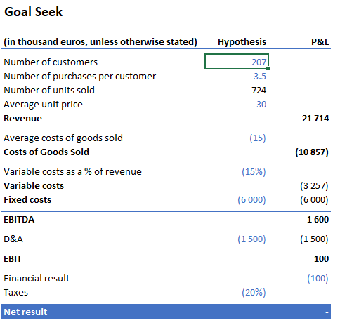
Let’s dive into a practical example to see just how helpful it can be:

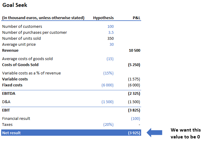
  • Let’s say you want to compute the minimum number of customers you need to have to be profitable (net result greater than 0);
  • the number of customers is an input among other inputs like the average unit price of your products, the average costs of goods sold, the variable costs and the fixed costs ;
  • the net result is the revenue – costs of goods sold – variable costs – fixed costs – depreciation & amorization – financial result – taxes.

To use Goal Seek, and find the minimum number of customers:

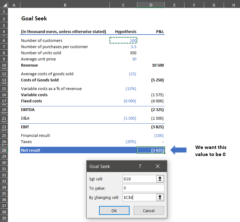
  • Navigate to the cell where you want the result to be zero.
  • Click on Data > What-If Analysis > Goal Seek (or hit Alt > A > W > G).
  • Set the “To value” as 0.
  • Specify the cell containing the number of customers under “By changing cell,” then hit OK.

Voilà! You now have the magic number of customers required to reach profitability.

In general, if you have multiple inputs, complicated formulas that give an output and you want to know the value of an input to reach a given value for an output, Goal Seek is your way to go.

VLookUp is Dead ! Long live XLookUp !

I’m sure you know VLookUp but have you met its more versatile cousin XLookUp ? If you try it, you’ll never use VLookUp again.

Why? Well, let me enlighten you:

  • Left-Side Retrieval: You can retrieve a value which is on the left of the looked up value ;
  • No Column Counting Needed: No need to count the number of columns ;
  • Auto-Adjusting Formula: If you add or delete a column, XLookUp will gracefully adapt.

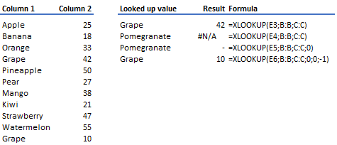
Here is how to use it :

=XLOOKUP(E3;B:B;C:C)

If you want the value to be 0 in case the looked-up value is not found, just add 0 at the end of the formula:

=XLOOKUP(E3;B:B;C:C;0)

But wait, there’s more. You can even reverse the lookup, scanning from bottom to top:

=XLOOKUP(E3;B:B;C:C;0;0;-1)

As I said, you’ll never use VLookUp again!

A Must-Have Macro : # ##0;(# ##0);- format

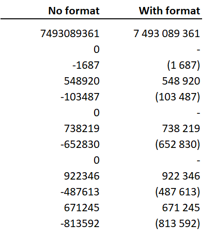
In the image below, the same list of numbers is presented in two columns :

  • On the left column, no particular format is applied ;
  • On the right column, a format where thousands are separated by a space, negative numbers are within brackets and zeros are “-” is applied.

Personally, I find the right column to be so much easier to read. I use this format so often that I have a Macro. Here’s how you can have it too :

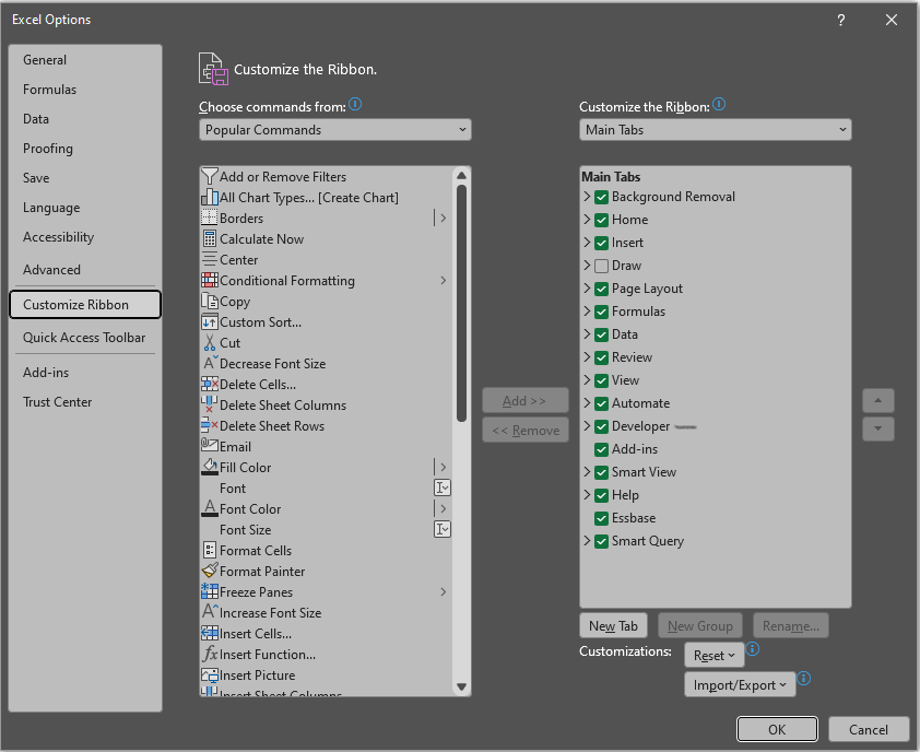
  • First, add the developer tab : File > Options > Customize Ribbon and check Developer

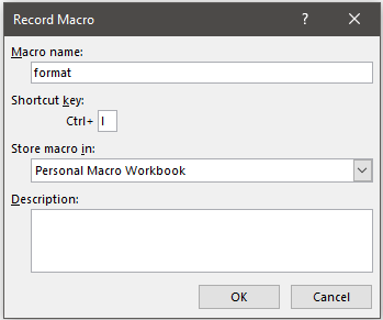
  • Second, record the Macro : Developer > Record Macro. Set the name and the letter lowercase L to launch the Macro using Ctrl+L. Make sure to select “Personal Macro Workbook” so that the Macro will be available across all Excel files :

  • Third, edit the format of whichever cell you are on by doing this and only this : right-click > Format Cells > Custom > # ##0;(# ##0);- > Ok > Developer > Stop Recording

Now you are set. Just do Ctrl+L to change the format. If you want to check the Macro you have recorded you can do Alt + F11 and on the left, go to “VBAProject (PERSONAL.XLSB)” > Modules > Module 1. You should see a code like this :

Sub format_1()
'
' format_1 Macro
'
' Keyboard Shortcut: Ctrl+l
'
    Selection.NumberFormat = "#,##0;(#,##0);-"
End Sub

Sum of visible cells only

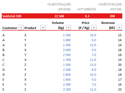
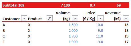
If you want to play with filters and see the results of the sum of a column, just add on top a subtotal(109;range) formula to see the sum of the visible cells only.

It is as effective as it is simple.

Rule #1 – Constants should be Blue

In Excel, we all have to deal with constants. Whether it is the number of customers, a price or the number of employees, they are constants. We call them constants but they can be seen as parameters. I propose making them all blue. It takes only a few seconds and can spare you a lot of trouble. In the sea of black formulas, blue constants stand out like beacons of clarity, guiding you through the intricate maze of data with ease.

On the contrary : revenue, costs, cash, are all calculated using a formula and should remain black.

Here is why :

  • If you go back to your Excel file some time later, you will instantly discern what can be tweaked and what must remain untouched
  • If you want to simulate results while changing the parameters, it is much quicker and easier to spot what can be changed
  • If the file is used by multiple persons, it prevents for putting a value on a cell containing a very complex formula. What’s worse than redoing what has already been done?

Here is an example : on the left, we cannot make the difference between constants and formulas. On the right it is as clear as it can be :

What happens if you don’t follow this rule :

  • People will take more time to understand how the file is working
  • You may be subject to someone erasing a formula for putting a raw value
  • It shows other people you are not used to very complex Excel files

So, let’s embrace the artist within and paint our constants blue. Let’s illuminate the path to clarity and efficiency in the realm of spreadsheets. After all, in the world of Excel, a stroke of color can make all the difference.