Automating Your Excel Files

Automating your Excel files can save you time and streamline your workflow. Here’s how to do it:

  1. Structure Your File: Organize your file into three main sections: Outputs, Analysis, and Inputs. This helps maintain clarity and organization. Refer to this post.
  2. Respect Rule #1: Use blue for parameters to easily identify and differentiate them from other data. Refer to this post.
  3. Formula-Based Computation: Anything that can be computed should be computed with a formula so that you never have to think about it again (even text such as the month in letters).
  4. Avoid Editing Sources: Instead of directly editing original sources, add formulas on the left or the right, even to deal with exceptions. This preserves data integrity and simplifies updates.
  5. Utilize Mapping Tables: When necessary, use mapping tables to standardize data or perform lookup operations.
  6. Eliminate Copy-Pasting: Try to avoid copy-pasting data. Instead, use formulas or data extraction with the use of pivot tables.
  7. Avoid manually entering data into cells whenever possible: It should be extracted from an Excel source whenever possible.
  8. Automate Error Checking: Use formulas to automate error-checking processes, ensuring data accuracy and consistency.
  9. Organize Data: Maintain data in list format to facilitate sorting, filtering, and analysis using pivot tables.
  10. Consider Macros: Explore the use of macros for repetitive tasks or complex operations. For instance, it can be used to send a pdf file to multiple recipients.

By following these guidelines, you can automate any Excel file, making updates and adjustments a breeze, requiring only to update some parameters and the inputs.

Should you automate your Excel Files ?

Whether it’s for daily, weekly, or monthly tasks like revenue analysis, margin tracking, or cash flow forecasts, automation can be a game-changer.

Some may argue that manual work helps uncover errors or aids in analysis, but I see it differently. Automating your files offers numerous benefits:

  • Deep understanding: Automating forces you to grasp the intricacies of your processes, including handling exceptions.
  • Time savings: You’ll save a lot of time, for sure. Time that can be dedicated to being a business partner, doing non recurring analysis that will make your company move forward (which is not the case with recurring analysis).
  • Delegation Ease: Automated files are easier to delegate, freeing up even more of your time.
  • Continuous Improvement: With automation in place, you can continuously refine and enhance your files. This will allow to push further the analysis.
  • Fastest Way to the End Result: You’ll get faster to the end result and you will spot with more ease potential mistakes. Then, and only then, you need to go into the details.

So, the next time you open a familiar Excel file, consider automating it step by step.
Tomorrow we’ll see exactly how to do it.

Excel Formula Tracking Tips

Dependents:

  • To check if data is used in a formula elsewhere, go to Formulas > Trace Dependents (Alt > M > D).
  • This can be particularly useful when you want to make sure you have correctly used an hypothesis in a business plan or a budget for instance.

Precedents:

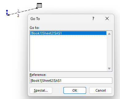
  • If you’re in a cell with a formula and want to identify its dependencies, try Formulas > Trace Precedents (Alt > M > P). It helps locate sources, especially across different sheets (double-click on the dashed arrow)

    Removing Arrows:

    • When you’re done, remove arrows using Formulas > Remove Arrows. (Alt > M > A > Enter)

    Custom Excel Settings

    If you’re into tweaking Excel to your liking, here’s my personal setup:

    Go to File > Options (Alt > F > T) :

    • General > Font size: 9
    • Advanced > After pressing Enter, move selection: Unchecked
    • Advanced > Decimal separator: Dot
    • Advanced > Thousands separator: Space
    • Formulas > Error checking rules: All unchecked
    • Don’t forget to add the Developer tab if you want to record macros: Customize Ribbons: Check “Developer”

    It’s not a must-do, but whenever I fire up Excel, I quickly set it up this way.

    Feel free to play around with colors too (General > Office Theme)

    Analyzing Revenue Variations

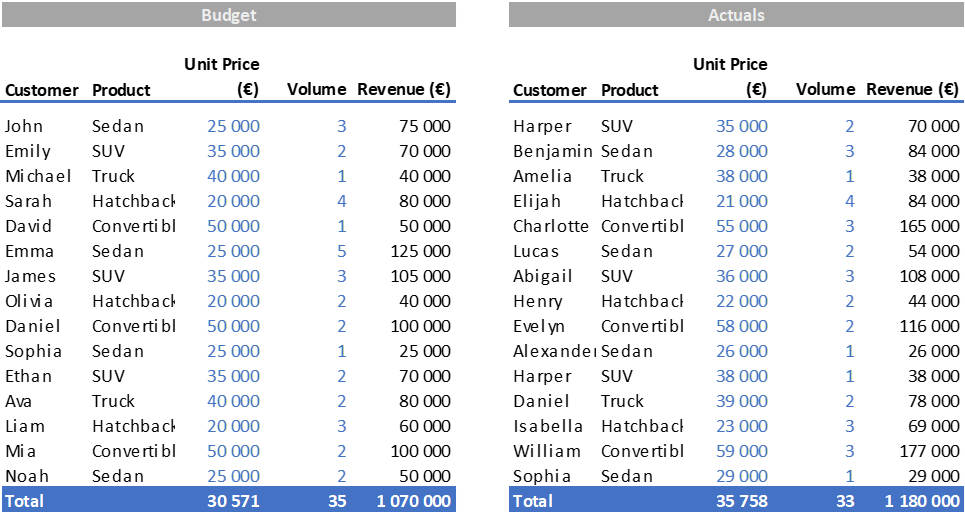
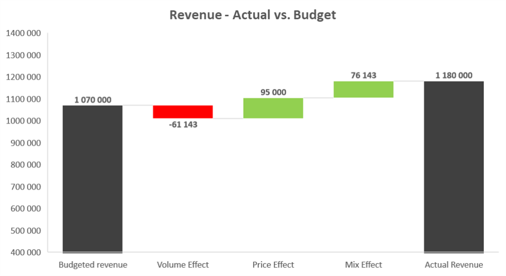
    Let’s say your revenue budget for last month was €1,070k, but you exceeded it by €110k. Now, you need to explain the main reasons for this variation to your shareholders.

    Here’s how to break it down:

    • Volume Effect:
      Calculate the difference between actual and budgeted volumes, multiplied by the budgeted unit price
    (Actual Volume - Budgeted Volume) * Budgeted Unit Price
    • Price Effect:
      For each product, compute the difference between actual and budgeted unit prices, multiplied by actual volumes. Sum up the price effects for each product. Bear in mind not to add a price effect for a product if the Budget did not anticipate this product to be sold.
    ΣAll products (Actual Unit Price - Budgeted Unit Price) * Actual Volume if Budgeted Unit Price ≠ 0
    • Mix Effect:
      Determine the overall price effect minus the sum of price effects for each product. This reveals the impact of changes in product mix.
    (Actual Unit Price - Budgeted Unit Price) * Actual Volume - Price Effect

    Now that you have the figures, focus on explaining the significant impacts only.

    Here’s an example to illustrate:

    Now you can explain the price effect of the convertible model (impact of +€58k) and the mix effect due to you selling more convertible models (which has the higher unit price) than expected (8 vs. 5).

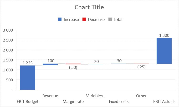
    Bridge in Excel (waterfall)

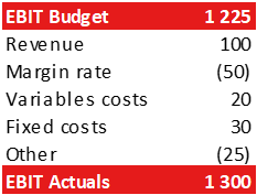
    Ever needed to compare two results, like EBIT or net sales, and explain the variations between them? That’s where a bridge comes in handy!

    Here’s how to build one:

    • Create a table: Start with a table that lists the starting point on the first row, the end point on the last row, and the various variations in between. You may need an “Other” line to ensure the bridge is complete.

    • Insert the Bridge: Select the table, go to Insert > Waterfall (Alt > N > I1 > Enter)

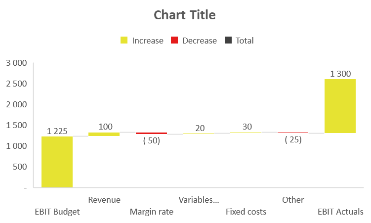
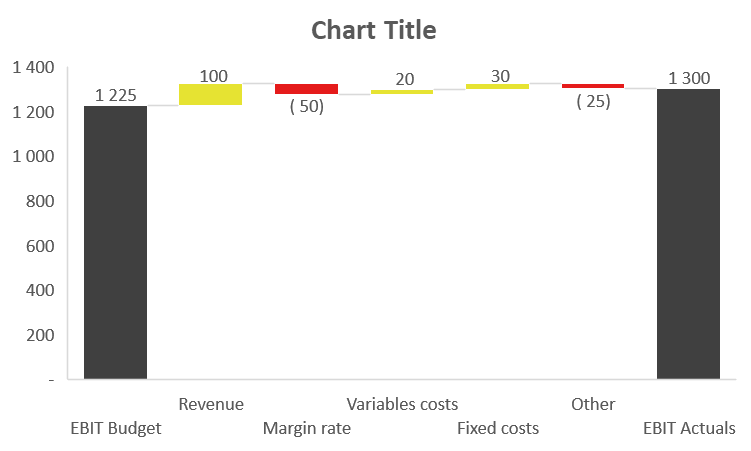
    • Customize the Appearance: Set the title in bold, delete the gridlines and borders (Alt > JA > SO > N > Enter). Change the colors in the legend to green for increase, red for decrease, and dark gray for total.

    • Final Touches: Delete the legend. Double-click the first and last columns, then right-click > Set as Total. You should obtain something similar to this:

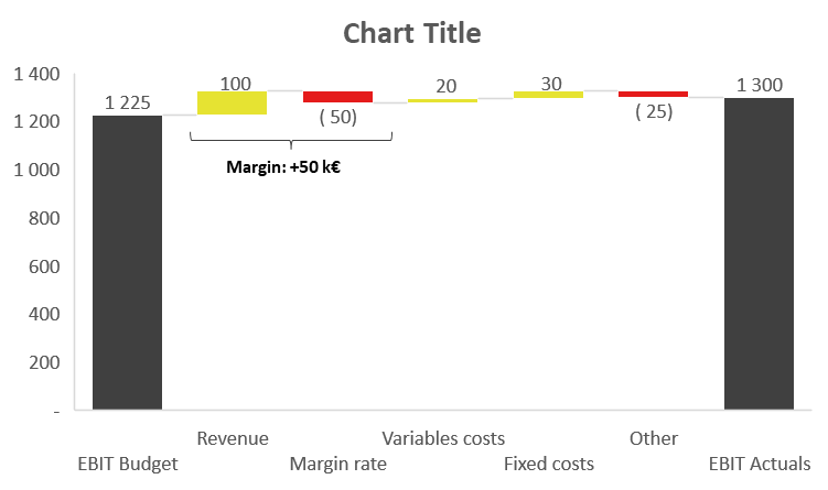
    You can now copy the bridge image into PowerPoint, position it on the left, and add commentaries on the right. For specific comments, consider adding brackets such as in the example below:

    Open a second Excel window

    This tip can save you a lot of time and headaches.

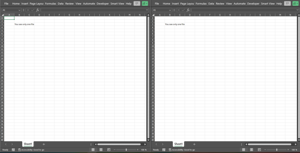
    Let’s say you have an Excel file with 50 sheets, and you want to work on a formula in the first sheet using data from the last sheet. Navigating between sheets can be cumbersome. Creating a new instance of the same Excel file allows you to switch back and forth between sheets easily. Here’s how to do it:

    • Go to View > New Window (or press Alt > W > N).

    Now, it’s like you have two instances of the same Excel file open. On one instance, go to the first sheet, and on the other, go to the last sheet.

    And here’s where the magic happens: you can simply press Alt + Tab to switch between sheets.

    You can even open more than two windows of the same Excel file. I use this all the time.

    Insert a table in a PowerPoint

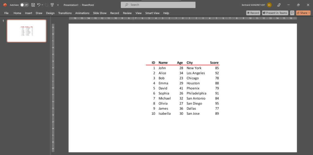
    You’ve worked on a table and want to insert it nicely into your PowerPoint. Here’s how to do it:

    1. In Excel, select the table and copy it.
    2. In PowerPoint, Home > Paste > Image (or Alt > H > V > U).

    Once pasted, never resize the image from the left/right or top/bottom sides, as this will distort the image ratio and make it look unappealing. Instead, always use one of the four corners or use Shift + Up/Down Arrow or Shift + Ctrl + Up/Down Arrow for increased control over the image size.

    There are other ways to insert a table in PowerPoint, but this method has never failed me.

    Rule #2: Never use merge

    If you want to merge two cells, please don’t do it!

    Merging cells prevents selecting individual rows or columns with Ctrl + Space or Shift + Space and can make pasting data trickier.

    But what if you want to center text across multiple cells? Do this instead:

    • Write the text in the cell on the left
    • Select the cells
    • Right-click > Format Cells > Alignment
    • In “Horizontal”, select “Center across selection”

    Here is the result:

    The Foundation of an Excel File

    Ever feel lost in all those sheets? Don’t worry, I’ve got your back. Let’s learn how to organize everything smoothly and efficiently. Ready to dive in?

    When faced with the task of creating an Excel file with numerous sheets, I recommend organizing them into distinct categories:

    • Inputs: This is where you store all the essential data. Always specify the data source to facilitate updates or inquiries.
    • Intermediary analysis: Here, calculations take place without the intention of presentation. It can be useful in complex excel files but they are not always needed.
    • Outputs: This is where you showcase your results.

    Set the color of tabs of the same category identical.

    Adopting this structure enhances clarity and simplifies workflow.

    Keeping calculations separate from raw data not only streamlines the Excel file but also makes it easier to update and comprehend by others.