Mastering Dynamic Summing in Excel with OFFSET and MATCH

If you need to sum a variable number of cells, such as calculating a year-to-date total for a monthly budget (e.g., from month 1 to month 5), here’s an efficient way to do it.

Step 1: Define Your Parameter

Start by defining the parameter. This could be the month number or the last day of the month, from which you can extract the month number using the formula MONTH().

Step 2: Use the SUM and OFFSET Functions

To achieve this, combine the SUM function with the OFFSET function. Here’s how OFFSET works:

  • Offset: You provide a reference range, and OFFSET shifts the starting point by a specified number of rows or columns.
  • Size Constraints: You can also define the number of rows and/or columns to include in the new range, which is key for our situation.

Example:

Here’s how it looks in action:

Let’s have a look at the formula :

There are certainly other ways to achieve this, but this method works well and is straightforward. Do note that you’ll need an up-to-date version of Excel to use the OFFSET function.

Going Deeper:

To make it more dynamic, you can also use the MATCH function to select a specific category, such as “Commerce” instead of “Marketing.” This adds flexibility, allowing you to fine-tune what data you want to sum.
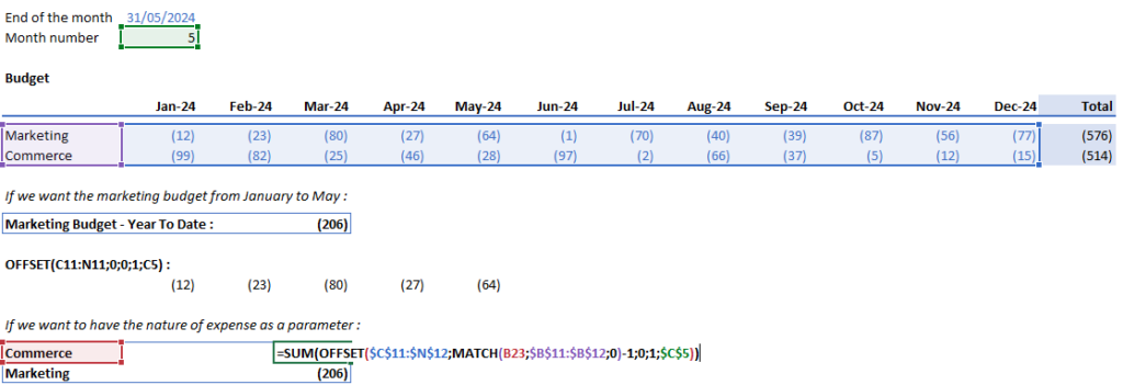
This proves to be useful when you want to compare year-to-date Actuals with year-to-date Budget at the end of a month.

Adjust a monthly budget in a second

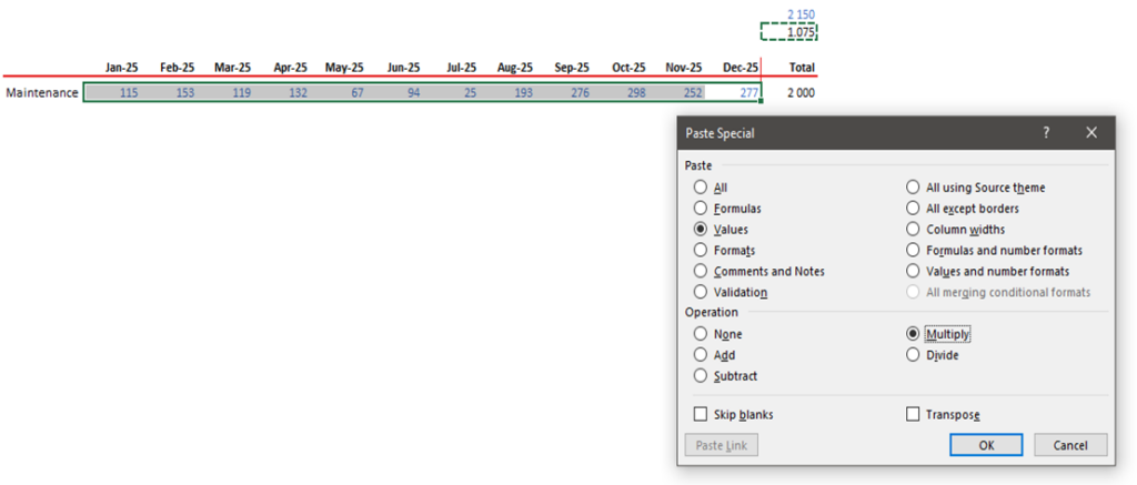
Sometimes you need to adjust a monthly budget for a certain item. For instance, let’s say you want to change the total budget from €2,000k to €2,150k.

Here’s a quick way to do it:

  1. Calculate the Adjustment Factor: Compute the ratio of the new total to the old total:

Adjustment Factor = 2,000 / 2,150 = 1.075

  1. Copy the Adjustment Factor: Copy the cell containing the value 1.075.
  2. Select the Monthly Budget Cells: Highlight the 12 cells that contain the monthly budget values.
  3. Apply the Adjustment Factor:
    • Right-click on the selected cells.
    • Choose Paste Special > Paste Special.
    • In the dialog box, select “Multiply” and “Values”.
    • Click OK.


By multiplying all the monthly budget cells by 1.075, your annual budget will be adjusted to €2,150k:

The Various Ways to Value a Company

This is the first post in a series about company valuation. We’ll start by exploring the different methods to value a company and then dive deeper into each one.

Method 1: The Discounted Cash Flow (DCF) Method

The DCF method views the company as a cash flow machine. Here’s how it works:

  1. Forecast the Cash Flow: Project the company’s future cash flows.
  2. Discount the Cash Flow: Apply the WACC (Weighted Average Cost of Capital) to discount the projected cash flows.
  3. Sum the Discounted Cash Flows: Sum these discounted cash flows over a specific period to determine the Enterprise Value.

If you’re unfamiliar with WACC, don’t worry—we’ll cover it in more detail later.

This will give you the Enterprise Value. If you want the Equity Value, you will need to substract the Net Debt (which is Debt – Cash and cash equivalents).

Equity Value = Enterprise Value - Net Debt

Method 2: The Multiple Method

This method involves comparing the company to others, either with historical purchase of companies known to the public or with publicly traded companies:

  1. Find Comparable Companies: Look for publicly known historical purchases or publicly traded companies.
  2. Determine Multiples: Calculate the Enterprise Value of these companies (Equity Value + Net Debt), then derive an EBITDA or EBIT multiple.
  3. Apply the Multiple: Use this multiple to compute the Enterprise Value for the company in question.
  4. Calculate Equity Value: Subtract the Net Debt from the Enterprise Value to get the Equity Value.

Method 3: The Balance Sheet Approach

For companies that don’t generate significant cash, their value might lie in their assets:

  1. Assess Assets: Evaluate the market value of the company’s assets, including brands, tangible assets, intangible assets, patents, or shares in other companies.
  2. Sum the Asset Values: Add up the market value of all assets.
  3. Subtract Liabilities: Subtract the total liabilities from the sum of the asset values to get the company’s value.

We won’t delve deeply into this method as it heavily depends on the specific company and the market value of its assets.

Divergent Results

When valuing a company using the DCF and Multiple methods, you might get different results. It’s crucial to understand why there are discrepancies rather than just averaging the outcomes from both methods.

Stay tuned for more detailed posts on each valuation method!

SUMIFS on both columns and rows

When you have criteria that apply to both rows and columns, summing elements based on these criteria can be a bit tricky. Here’s an example to illustrate this:

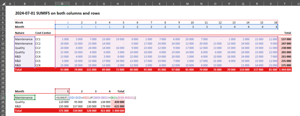
Imagine you want a summary of data month by month for each category (Nature). You need to check the criteria both on the Nature column and the Month row. Here’s how you can do it:

The Formula

=SUM(IF($D$5:$S$5=D$21;IF($B$9:$B$15=$B23;$D$9:$S$15)))

This formula will give you the desired summary:

Breaking It Down

To understand how this works, consider the formula without the SUM function:

=IF($D$5:$S$5=D$21;IF($B$9:$B$15=$B23;$D$9:$S$15))

This formula will return a new range based on your criteria:

  1. $D$5:$S$5=D$21: Checks if the values in the month row match the specified month.
  2. $B$9:$B$15=$B23: Checks if the values in the nature column match the specified nature.
  3. $D$9:$S$15: Refers to the data range you want to sum.

Will give you a new range:

When you sum this new range, you will get the total for the specified nature and month. For example, this will give you the sum of the maintenance for the 1st month, exactly as expected.

Example Summary

By applying this formula, you can create a summary table like the one below:

Use this technique to effectively sum data with multiple criteria across both rows and columns.

Debt amortization

Understanding how to compute the monthly reimbursement amount of a debt is crucial for financial planning. Let’s explore two methods to achieve this:

Method 1: The Formula

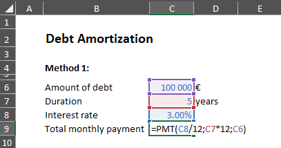
Using a straightforward formula, you can easily calculate the monthly reimbursement amount.

Méthode 2: Debt Amortization Schedule

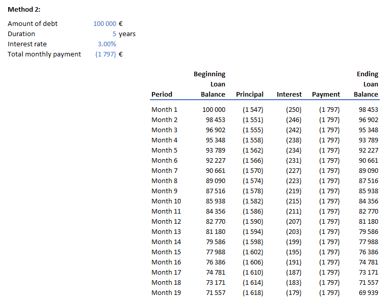
This method involves computing the amount of capital reimbursed and the interest paid each month. Let’s create a table with headers and rows for each month (N = 60 for a 5-year term). The table will have six columns:

  • Period: Sequential month number
  • Beginning Loan Balance: Ending balance from the previous month
  • Payment: Total Payment – Interest
  • Interest: Calculate the interest paid
  • Total Payment: we will find the correct value using Goal Seek
  • End Loan Balance: Beginning balance minus the capital reimbursed

See below the formulas for each column:

To find the monthly reimbursement amount of €1,797, we use the Goal Seek function. Set the capital due to zero at the end of the period, and let Goal Seek adjust the monthly reimbursement amount accordingly.

With these calculations, you can simulate the financial results for any given period. For a P&L simulation, consider the interest paid. For cash flow or balance sheet simulations, use both the capital reimbursed and the interest paid.

Note: If you have a grace period (e.g., 6 months without payments), you can easily incorporate this into your simulation.

EBITDA, EBIT, Free cash flow and Cash flow

EBITDA: Earnings Before Interest, Taxes, Depreciation and Amortization

EBITDA = Revenue – Costs of Goods Sold – Variable Costs – Fixed Costs (excl. depreciation and amortization of fixed assets, financial results and income taxes)

It is often used when we want a short answer to the question “How much this company is valued?” It depends on the company’s industry but a number we often multiply the EBITDA by 7 to get the Enterprise Value. This gives you:

Equity Value = Enterprise Value - Net Debt with Enterprise Value = 7 * EBITDA and Net Debt = Debt - Cash and cash equivalents

EBIT: Earnings Before Interest and Taxes

EBIT = EBITDA - Depreciation and Amortization of fixed assets

Free cash flow: Cash flow from Operations less Capital Expenditure.

It is cash flow that can be dedicated to the reimbursment of debts, paying of dividends, …

Free cash flow = EBITDA - Change in Working Capital - Income Taxes - Investments

Cash Flow: The variation of cash from one period to another, resulting from operating activities, investments and financing activities.

Cash flow = Free cash flow - financing activities (reimbursment of debts, funding, …)

Let’s see an example:

Mastering F5 in Excel

Pressing F5 in Excel allows you to navigate to specific cells and select certain cells based on criteria. Let’s break it down:

Navigate to a Cell

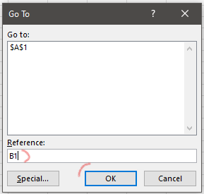
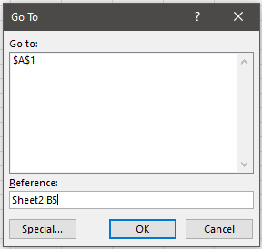
Simply press F5 and enter the cell reference to swiftly move to a specific cell.

Select Specific Cells

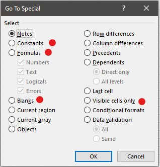
Click on “Special” to access a range of selection criteria. Here are some commonly used ones:

  • Constants: select only cells containing a value, for instance to color them all in blue
  • Formulas: select only cells containing a formula
  • Blanks: select only blank cells
  • Visible cells only: When filtering data, this option selects only the visible cells. Very useful if you want to paste a formula to filtered cells only

Mastering F5 empowers you to efficiently navigate and manipulate data in Excel.

The various ways of pasting in Excel

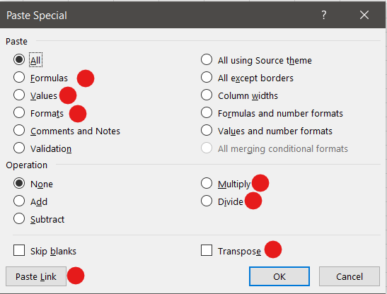
In Excel, pasting isn’t always as straightforward as pressing Ctrl + V. By right-clicking and selecting “Paste Special,” you can access a range of pasting options.

Let’s explore the most commonly used types of pasting:

  • Formulas: Pastes the formula only.
  • Values: Pastes the value without the formula.
  • Formats: Pastes the format only.
  • Multiply: Multiplies the content in the cell by what was copied.
  • Divide: Divides the content in the cell.
  • Transpose: Converts a row into a column or vice versa.
  • Paste Link: Inserts a link to the copied cell. Very useful when combined with the method of using another window of the same Excel file.

These are the fundamental pasting methods you’ll find yourself using frequently in Excel.

Margin Variance: Revenue/Volume Effect, Price Effect, Costs Effect, Mix Effect

Explaining a margin variation between actual and budgeted results for last month is essential. While we’ve discussed how to explain revenue variation previously, let’s delve into margin variance.
There are several approaches, but here’s what I find most useful:

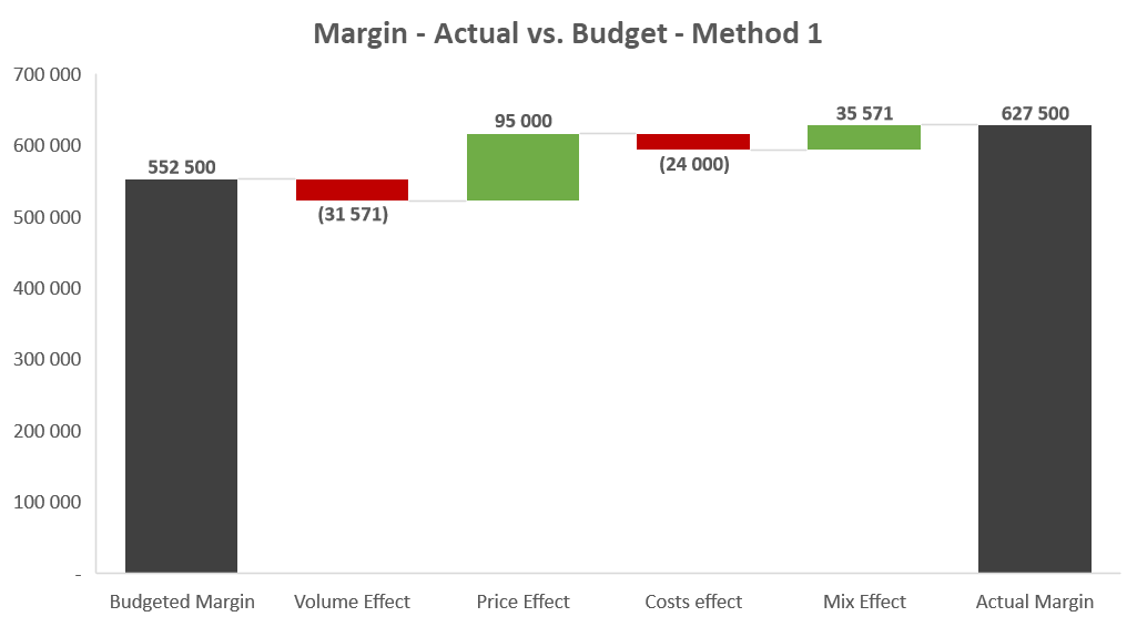
  • Method 1: Volume & Unit Margin
Volume Effect = (Actual Volume - Budgeted Volume) * Budgeted Unit Margin
Price effect = Sum of Price Effect on all products
Costs effect = Sum of Costs Effect on all products
Mix effect = (Actual Unit Margin - Budgeted Unit Margin) * Actual Volume - Price effect - Costs effect
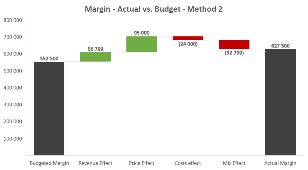
  • Method 2: Revenue & Margin Rate
Revenue Effect = (Actual Revenue - Budgeted Revenue) * Budgeted Margin Rate
Price effect = Sum of Price Effect on all products
Costs effect = Sum of Costs Effect on all products
Mix effect = (Actual Margin Rate - Budgeted Margin Rate) * Actual Revenue - Price effect - Costs effect

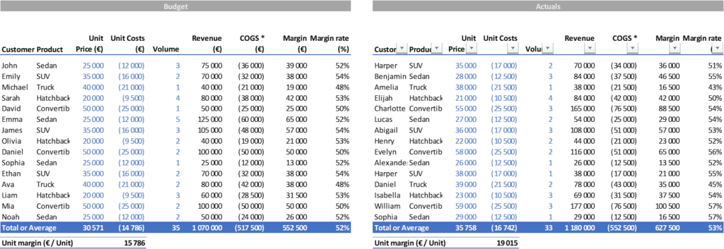
Let’s examine an example using both methods:

What can we infer from this example?

  • Both methods yield different results as the volume is lower (-2 cars) and the revenue higher (+€110 k)
  • Method 1 is more representative for a range of similar products with unit margins in a reasonable range. If you sell screws and nails along with cars, the second method will be more suitable.
  • Method 2 is preferable when dealing with products with varying unit prices, focusing on revenue and margin rate rather than volume and unit margin.

Some Basic Shortcuts in Excel: Select/Add/Remove Row or Column, Re-do Last Action

To select a row, press Shift + Space
For selecting a column, press Ctrl + Space. That’s when respecting the « never use merge » rule gets beneficial. If you’ve merged cells, using Ctrl + Space will select all merged columns—not what you want.

With a row selected, Ctrl + ‘+’ adds a new row, and Ctrl + ‘-‘ removes the selected one.

Similarly, for columns, Ctrl + ‘+’ adds a new column, and Ctrl + ‘-‘ removes the selected one.

Of course you also have Ctrl + C to copy, Ctrl + X to cut and Ctrl + V to paste, Ctrl + Z to cancel last action and Ctrl + Y to redo the last action canceled but these are not specific to Excel.

Press F4 to redo the exact same action you just performed. It can be adding color, inserting a row or anything you just did.

Use these shortcuts regularly, and they’ll soon become second nature.