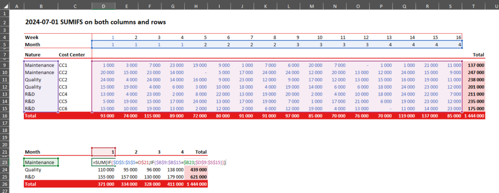
When you have criteria that apply to both rows and columns, summing elements based on these criteria can be a bit tricky. Here’s an example to illustrate this:

Imagine you want a summary of data month by month for each category (Nature). You need to check the criteria both on the Nature column and the Month row. Here’s how you can do it:
The Formula
=SUM(IF($D$5:$S$5=D$21;IF($B$9:$B$15=$B23;$D$9:$S$15)))
This formula will give you the desired summary:

Breaking It Down
To understand how this works, consider the formula without the SUM function:
=IF($D$5:$S$5=D$21;IF($B$9:$B$15=$B23;$D$9:$S$15))This formula will return a new range based on your criteria:
- $D$5:$S$5=D$21: Checks if the values in the month row match the specified month.
- $B$9:$B$15=$B23: Checks if the values in the nature column match the specified nature.
- $D$9:$S$15: Refers to the data range you want to sum.
Will give you a new range:

When you sum this new range, you will get the total for the specified nature and month. For example, this will give you the sum of the maintenance for the 1st month, exactly as expected.
Example Summary
By applying this formula, you can create a summary table like the one below:

Use this technique to effectively sum data with multiple criteria across both rows and columns.
