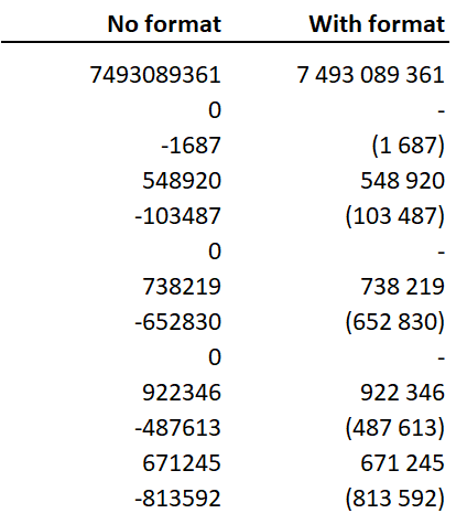
In the image below, the same list of numbers is presented in two columns :
- On the left column, no particular format is applied ;
- On the right column, a format where thousands are separated by a space, negative numbers are within brackets and zeros are “-” is applied.

Personally, I find the right column to be so much easier to read. I use this format so often that I have a Macro. Here’s how you can have it too :
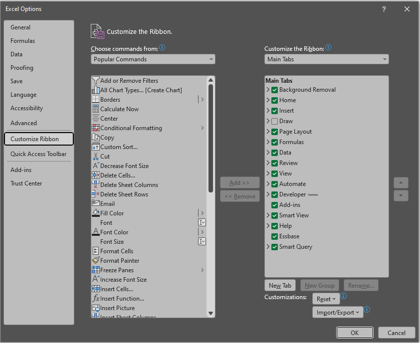
- First, add the developer tab : File > Options > Customize Ribbon and check Developer

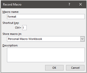
- Second, record the Macro : Developer > Record Macro. Set the name and the letter lowercase L to launch the Macro using Ctrl+L. Make sure to select “Personal Macro Workbook” so that the Macro will be available across all Excel files :

- Third, edit the format of whichever cell you are on by doing this and only this : right-click > Format Cells > Custom > # ##0;(# ##0);- > Ok > Developer > Stop Recording
Now you are set. Just do Ctrl+L to change the format. If you want to check the Macro you have recorded you can do Alt + F11 and on the left, go to “VBAProject (PERSONAL.XLSB)” > Modules > Module 1. You should see a code like this :
Sub format_1()
'
' format_1 Macro
'
' Keyboard Shortcut: Ctrl+l
'
    Selection.NumberFormat = "#,##0;(#,##0);-"
End Sub